TL;DR: I created a logic-based solver and generator for japanese arrow puzzles. You can try them at yazudo.app or check out the code.
The Puzzle
I came across the japanese arrow puzzles when reading Knuth’s TAOCP, Volume 4B on backtrack programming, which discusses applications of backtracking and dancing links to solve various kinds of puzzles. According to Knuth, those puzzles where first published in japanese puzzle magazines in the 90s.
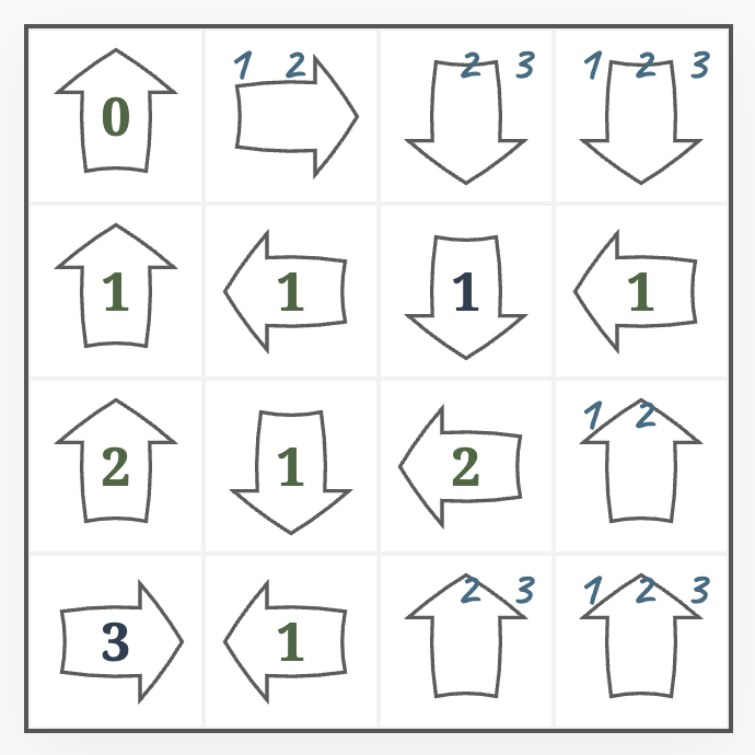
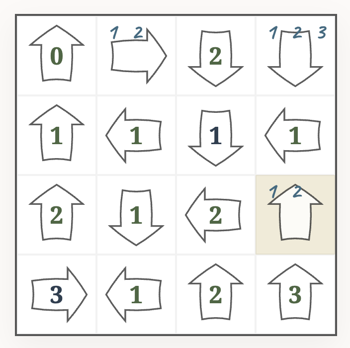
This kind of puzzle is played on a (usually square) grid of cells, where each cell contains an arrow pointing either horizontally, vertically, or (in some puzzles) diagonally. Some of the arrows may already contain numbers (the initial clues).
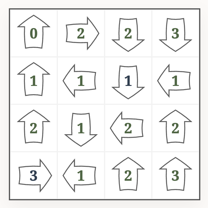
The goal is to write a number into each arrow, such that the number in each arrow corresponds to the count of distinct numbers in the cells that the arrow points at. For example, this is the solution of the above puzzle:
Although not officially a part of the puzzles rule, it is typically assumed that any well-formed logic puzzle has a unique solution. But whether this fact may be used in solving the puzzle is considered controversial by some players.
I set out to write an algorithm to generate these kinds of puzzles. However, not just any valid puzzles, they should have the right level of difficulty: not trivial, but also not too frustrating. But what does that even mean – when a puzzle is too frustrating to solve?
How Humans Solve Puzzles, as Opposed to Machines
It is not hard to solve the above puzzle using backtracking. An algorithmic solver could first enter candidates for each cell, based on the rules of the puzzle:
- if an arrow already sees
idistinct numbers, we can discard candidates<i - if an arrow has
icells ahead, we can discard candidates>i
In the above example puzzle, this leads to something like this:
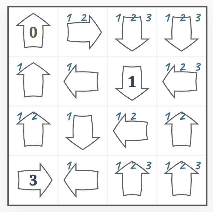
And after filling out cells with just one clue (the “naked singles” in Sudoku terms), we have
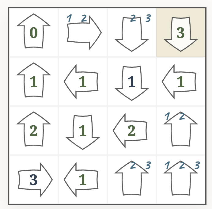
Next, the backtracking solver would guess a candidate for one of the free cells to continue. For example, we could guess that the top right cell is a $3$:
After applying the basic rules, we again have to guess. Let’s say the free cell at the bottom is also a $3$.
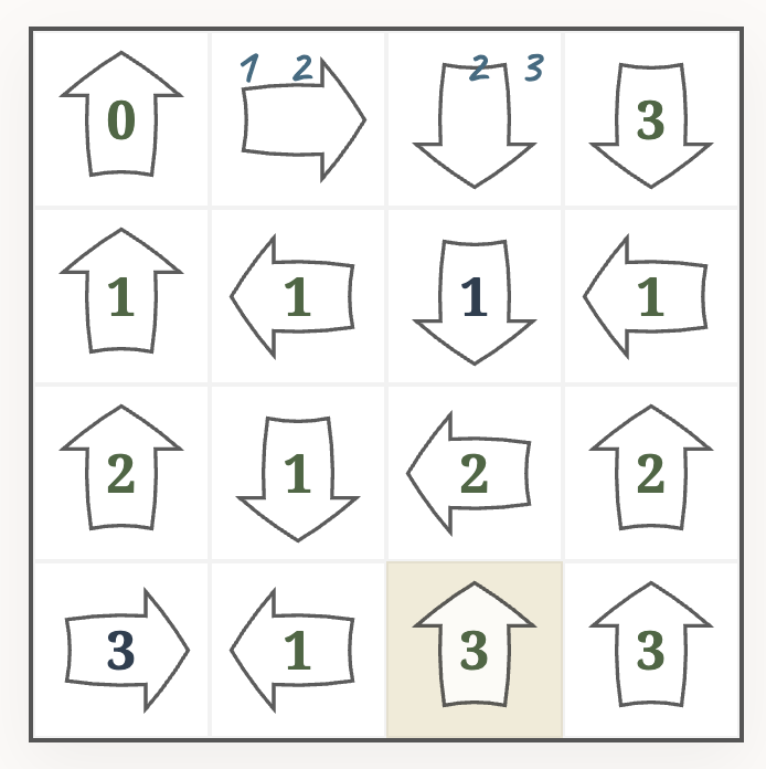
Now we have reached a contradiction: the cell in the bottom left corner says $3$, but the arrow sees only two distinct numbers. That means, one of our guesses must have been wrong. We need to backtrack – at least to the state before guessing the $3$ in the bottom row – and try a different number, until we succeed.
This is how a computer would solve the puzzle. But in my opinion, humans approach such puzzles very differently. And in fact, this backtracking approach is often considered unfun, or essentially “guessing” - not solving the puzzle with logic. Ultimately it is also just hard to execute for humans, as you need to keep a stack of the undoable actions in your mind – and humans have very limited working memory.
So, do humans simply not use backtracking? I think this is also not entirely true, but they apply it only in limited fashion. But then, how do humans solve puzzles? I can’t speak for all of them; but I can illustrate, how I would approach the above puzzle.
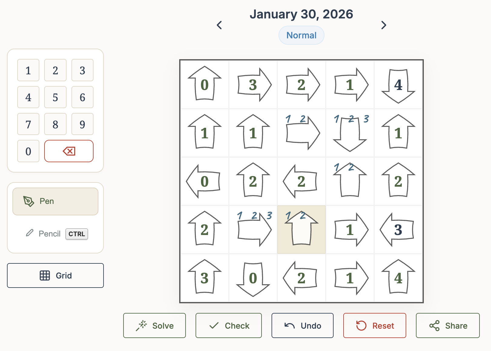
After filling in the obvious elements, we are at
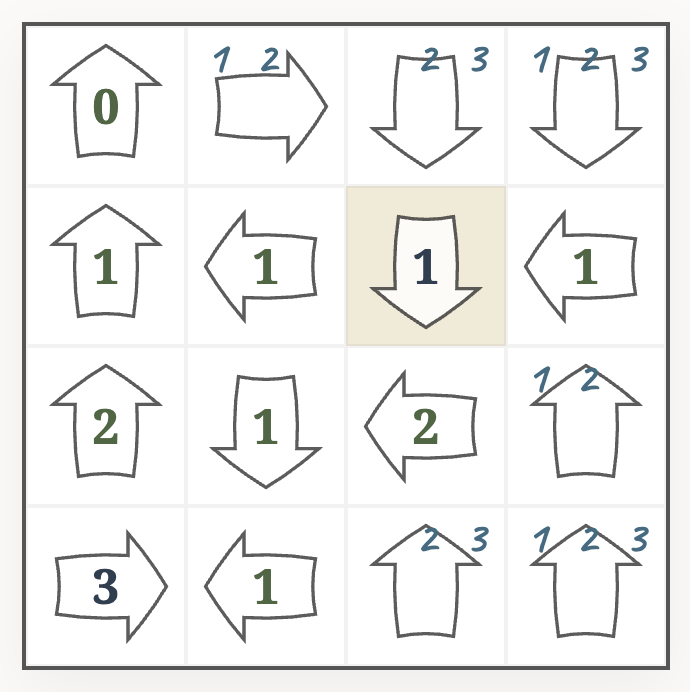
Next, we can apply a logical deduction that follows from the basic rules of the puzzle. The arrow in the marked cell has a $1$, and already sees a $2$. That means, the cell below in the bottom row must also be a $2$.
After applying a few more rules of this kind, we may end up in this state.
What should be the value of the marked cell? One way to continue is to do a short proof by contradiction:
- Assume that the marked cell is a $1$.
- Then the cell in the top-right corner is also $1$.
- This contradicts the $3$ in the bottom-right corner.
- We can conclude that our assumption was wrong, and the marked cell must be the only other candidate ($2$).
But wait, isn’t that line of thinking essentially backtracking? Yes, but only in a very limited fashion. We have guessed only one number (not repeatedly), and then focused again on applying logical rules until we hit a contradiction.
To conclude, my hypothesis is that
- Humans mostly use logical rules to solve the puzzle. These rules are derived from the basic rules of the puzzle, but can be much more complex. In fact, logic puzzles can be considered elegant or beautiful, if they allow such complex patterns to emerge out of a set of simple base rules. Typically, simpler rules are tried first, and once possibilities with those are exhausted, one continues with more complex rules.
- Once rules no longer yield progress, humans also employ a limited amount of backtracking. This typically amounts to only “guessing” one number, then applying a few further rules in their head to see if a contradiction is reached.
- Is that still does not lead to progress, deeper backtracking or “forcing” techniques may be applied. At least for me, this is usually where the puzzles feel more like a chore than entertainment, but your mileage may vary.
Why do we need to know all this, just to generate puzzles? The idea is, once we generate a valid puzzle (in whatever way), we try to solve it using the human way. If that’s not possible, the puzzle may rely too much on backtracking to be enjoyable.
We can also record which logical rules are required to solve the puzzle, and whether the limited proof-by-contradiction backtracking needs to be applied at all. Based on that, we can discard too easy puzzles, and obtain a difficulty rating for the others.
The Human-Like Solver
The general concept of a rule-based solver is simple. We try out all the rules and attempt to make progress (filling cells or at least eliminating candidates). Either we will end up with the solved puzzle, or a partially solved state where non of the rules make progress.
def solve(puzzle):
  progress = True
  while progress:
    progress = False
    for rule in rules:
      if rule.progress(puzzle):
        rule.apply()
        progress = True
        if puzzle.solved():
          return solution
  return UNFINISHED
For simplicity, we assume here that the puzzle is valid, i.e. it has exactly one solution.
So, how will we represent the rules? One simple approach would certainly be to implement one function per rule.
class Rule(ABC):

  @abstractmethod
  def apply(puzzle: Puzzle) -> Optional[Progress]
    pass
As an example let’s take this rule:
If two arrows are directly next to each other and point in the same direction, and the front arrow is filled with number
i, then the back arrow has either numberiori+1.
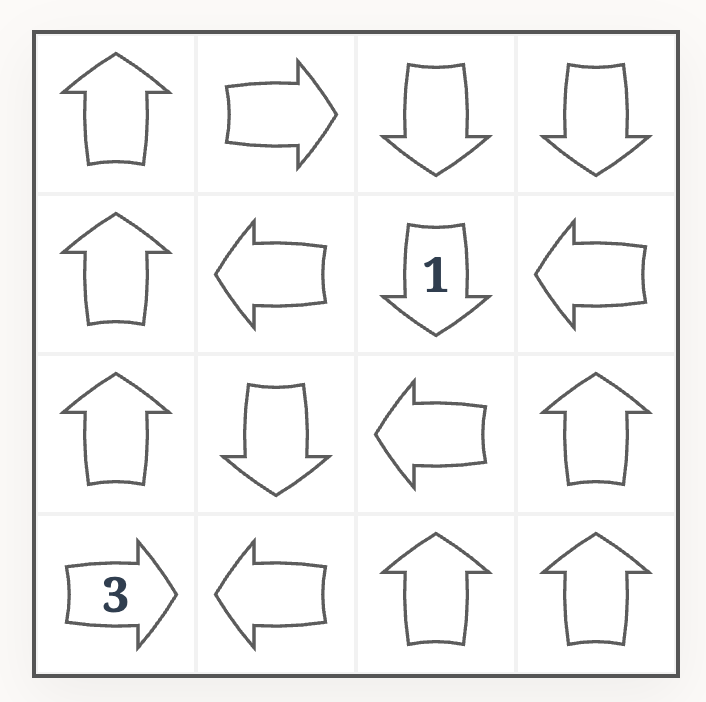
To illustrate this, take a look at the following puzzle. The marked arrow points at an arrow filled with a $1$.
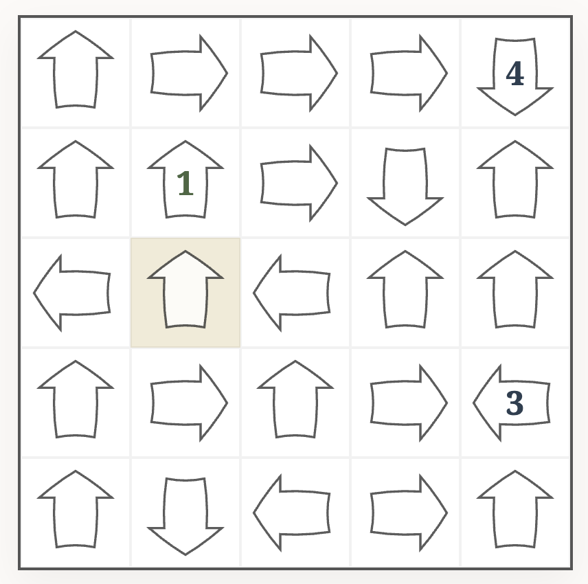
Either the cell in the top row is also a $1$, in which case the marked arrow is also $1$; or the cell in the top row is not a $1$, in which case the marked arrow is a $2$.
The rule could be translated into Python code like this
class NextArrowSameDirection(Rule):

  @override
  def apply(puzzle: Puzzle) -> Optional[Progress]:
    for cell in puzzle:
      next_cell = puzzle.next(cell)
      if next_cell is None:
        continue
      if next_cell.direction != cell.direction:
        continue
      if (i := next_cell.value) is None:
        continue
      return Progress(cell=cell, candidates={i, i+1})
    return None
In a puzzle with $n$ by $n$ cells, this rule takes $\mathcal{O}(n^2)$ time to check,
This approach would certainly work well. So why did I not follow it?
- It seems a bit inflexible, for fast iteration / prototyping, to always write or adapt code. Also, especially for more complex rules, the nested loops and conditions can get harder to read and feel quite detached from the actual rule idea.
- (and more importantly) I thought it would be much less fun than what I ended up doing instead. Which is…
Representing Rules Using Logical Formulas
In the end, we are writing logical rules, so why not represent them using logical formulas? I have decided to use first-order logic to represent the rules via conditions and conclusions. For example, for the above rule, the condition can be written as
\begin{equation} \exists p,q,i (\text{next}(p) = q \wedge \text{dir}(p) = \text{dir}(q) \wedge \text{val}(q) = i \wedge i \neq \text{nil}) \end{equation}
There are positions (cells) $p,q$ such that the arrow at $p$ directly points at $q$ ($\text{next}(p) = q$), the arrows at $p,q$ have the same direction ($\text{dir}(p) = \text{dir}(q)$) and the cell $q$ is already filled with $i$.
The conclusion is
\begin{equation} \text{only}(p, [i, i+1]) \end{equation}
The cell at $p$ can only be either $i$ or $i+1$.
The formal language applied is first-order logic (FO) with a set of relations and functions that are related to the puzzle structure, such as next, dir and val. Some other examples are
- the binary relation
points_at(p, q)which is true when $q$ can be seen (immediately or with other cells inbetween) by the arrow at $p$ - the function
sees_distinct(p)which is the count of distinct numbers currently seen by the arrow at $p$
So we could encode the constraint of a filled out japanese arrow grid being valid as \begin{equation} \forall p (\text{val}(p) = \text{sees_distinct}(p)) \end{equation}
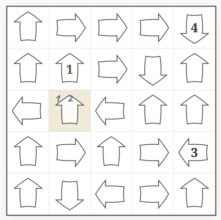
But how do we use these conditions and conclusions in the solver to apply rules? Each condition is a first-order formula with some existential quantifiers (e.g. $\exists p,q,i$ above). We are trying to find positions $p,q$ and numbers $i$ to make the formula true, essentially by trying all possible candidates until we find a witness $p,q,i$ that fulfills the conditions. Let’s look again at our example puzzle from above:
In this case (using $0$-based $(y,x)$ coordinates), we have $p = (2,1), q = (1,1), i = 1$.
We can then plug those values into the conclusion $\text{only}(p, [i, i+1])$ to obtain $\text{only}((2,1), [1, 2])$. That means the candidates of cell $(2,1)$ will be limited to $1$, $2$.
There is one thing I have so far only glossed over (actually, there are many such things – but I don’t want to bore you too much with all the details). When we write $\exists p,q,i$ we are actually quantifying over two different kinds of objects: $p,q$ are positions (or cells), and $i$ is a number. So, our Universe in which we evaluate objects actually contains several different kinds of objects, and in reality we have typed quantifers $\exists_{\text{pos}} p$ and $\exists_{\text{num}} i$ for each type. There is even a third type, the type of directions (e.g. used in $\text{dir}(p)$). Hence, functions also have types (for example, $dir$ is a function from positions to directions).
However, it would be awkward to write down formulas like this
\begin{equation} \exists_{\text{pos}} p,q \ \exists_{\text{num}}i \ldots \end{equation}
so we just write $\exists p,q,i$ and follow the convention that $p,q,r \ldots$ are position variables, and $i,j,k \ldots$ are numeric variables.
In our solver, the current (partially solved) puzzles naturally define a universe (the sets of positions, numbers and directions), as well as the relations and functions (such as points_at and val) that we can use to evaluate formulas. Applying a rule then boils down to model checking – proving that the condition is true by providing a witness for the existential quantifiers; and henceforth using this witness to apply the conclusion.
Implementing Model Checking
We now have a representation of logical rules as formulas (strings), but ultimately we need to end up with an interpreter of such formulas in the context of puzzles. That means, there is no way around going through the five stages of grief.
- Lexing
- Parsing
- Type Checking
- Optimization / “Code Generation”
- Interpretation
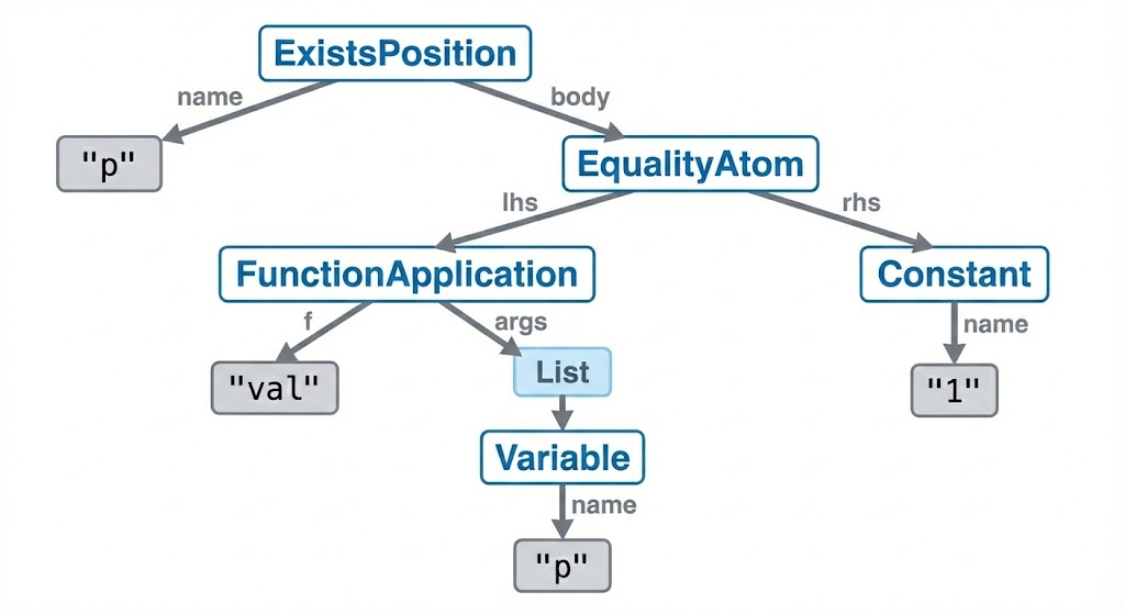
Lexing and Parsing bring us from a string representation like $\exists p (val(p) = 1)$ to an abstract syntax tree (AST) like
ExistsPosition(
  name="p",
  body=EqualityAtom(
    lhs=FunctionApplication(
      f="val",
      args=[
        Variable(name="p")
      ]
    ),
    rhs=Constant(name="1")
  )
)
Since variables are typed, it makes sense to type-check the parsed formula next to avoid some classes of semantic errors. For example, a formula like $\exists p (val(p) = dir(p))$ would parse but not type-check, as we are comparing numbers $\text{val}(p)$ with directions $\text{dir}(p)$.
Let’s skip optimization for now and jump straight to interpretation. We can recursively evaluate a formula using its AST in a straight-forward way: quantifiers become for-loops, conjunctions are translated to repeated if-statements, and so on. Our example rule
\begin{equation} \exists p,q,i (\text{next}(p) = q \wedge \text{dir}(p) = \text{dir}(q) \wedge \text{val}(q) = i \wedge i \neq \text{nil}) \end{equation}
then ultimately will be interpreted in a manner like this
for p in puzzle.cells:
  for q in puzzle.cells:
    for i in range(1, puzzle.dimension+1):
      if puzzle.next(p) != q:
        continue
      if puzzle.dir(p) != puzzle.dir(q):
        continue
      if puzzle.val(q) == i:
        return Witness(p=p, q=q, i=i)
return None
At first glance, not so different from our original Python implementation of the rule. But wait, we are now doing three nested for-loops, and the complexity has bumped up from $\mathcal{O}(n^2)$ to $\mathcal{O}(n^5)$! So this is painfully slow to check repeatedly. Which brings us to the step we skipped above:
Optimization
It is clear that the main pain point of evaluating formulas are the quantifiers (essentially for-loops). A simple technique we can use to reduce the “nestedness” of loops is to push quantifiers inwards (miniscoping).
In our example, we can push the $\exists i$ further in to reach \begin{equation} \exists p,q (\text{next}(p) = q \wedge \text{dir}(p) = \text{dir}(q) \wedge \exists i (\text{val}(q) = i \wedge i \neq \text{nil})) \end{equation}
As miniscoping is just an application of simple syntactic rules, it can be automated by the formula compiler, so we are actually not forced to write our formulas in this way.
This brings our evaluation code roughly to something like
for p in puzzle.cells:
  for q in puzzle.cells:
    if puzzle.next(p) != q:
      continue
    if puzzle.dir(p) != puzzle.dir(q):
      continue
    for i in range(1, puzzle.dimension+1):
      if puzzle.val(q) == i:
        return Witness(p=p, q=q, i=i)
return None
Since the inner loop over i will only run $\mathcal{O}(n^2)$ times, this brings the time complexity down to $\mathcal{O}(n^4)$. An improvement, but we can still do better!
Another promising approach is to completely get rid of quantifiers (quantifier elimination). In our example we require $\text{val}(q) = i$, so we can go ahead and remove $i$, as long as we replace all of its occurrences with $\text{val}(q)$.
\begin{equation} \exists p,q (\text{next}(p) = q \wedge \text{dir}(p) = \text{dir}(q) \wedge \text{val}(q) \neq \text{nil}) \end{equation}
Actually, there were other occurrences of $i$ in the conclusion \begin{equation} \text{only}(p, [i, i+1]) \end{equation} which becomes \begin{equation} \text{only}(p, [\text{val}(q), \text{val}(q)+1]) \end{equation}
It is a bit less obvious, but we can continue to also eliminate $q$! Since $\text{next}(p) = q$, our condition becomes
\begin{equation} \exists p (\text{dir}(p) = \text{dir}(\text{next}(p)) \wedge \text{val}(\text{next}(p)) \neq \text{nil}) \end{equation}
and the conclusion ends up as
\begin{equation} \text{only}(p, [\text{val}(\text{next}(p)), \text{val}(\text{next}(p))+1]) \end{equation}
We can finally model check this in $\mathcal{O}(n^2)$, as the interpretation will roughly execute
for p in puzzle.cells:
  if puzzle.dir(puzzle.next(p)) == puzzle.dir(p) and puzzle.val(puzzle.next(p)) != puzzle.nil:
    return Witness(p=p)
return None
However, the conclusion has become barely readable, and we certainly don’t want to write formulas this way! So we need to ideally automate quantifier elimination as well.
I didn’t really think about a sophisticated theory of when exactly we can eliminate quantifiers, as the following special instance essentially covered all of the relevant cases. Most rules have conditions of the form
\begin{equation} \exists x_1 \ldots \exists x_n \bigwedge_{i=1}^m \phi_i \end{equation}
If $\phi_j$ is an atom $x_k = t$ where $x_k$ does not appear in $t$, we can remove $\phi_j$, remove the quantifier $\exists x_k$ and finally replace every other occurrence of $x_k$ in the condition and conclusion with $t$.
With this approach we can automatically perform most possible quantifier eliminations in the compiler, but keep writing our formulas in the more readable way.
Here’s the impact of the optimizations on the runtime of the solver integration tests.
| Optimizations | Runtime |
|---|---|
| None | 4m47s |
| Miniscoping | 19s |
| Quantifier Elimination | 48s |
| Both | 9s |
Each optimization has – independently – a huge impact, but the performance still improves further significantly when combining both.
Backtracking
To complete our human-like solver, we need to implement also the limited backtracking, that will be applied when no rules can make any progress.
- Pick a cell and guess one of the candidates
- Apply a sequence of up to $k$ rules
- Check for a contradiction to the japanese arrow constraints.
If a contradiction is found, the guess was wrong $\Rightarrow$ eliminate the guessed candidate from the picked cell.
Increasing $k$ will increase the solver runtime exponentially, as we need to do a DFS or BFS of depth $k$ over the graph of possible rule applications. This limits the size of the puzzles that can be solved – and hence generated – in a reasonable timeframe. But thankfully, to mimic human abilities, $k$ should typically be a small number. I have mostly used $k=1$ or $k=2$.
Based on that, we can have programmatic $k$-solvers of different strengths to mimic human solvers of different skill levels
- $k=0$, i.e. no backtracking
- $k=1$, guess and think ahead one step
and so on.
Generating Puzzles
With the solver finally out of the way, the basic approach for generating puzzles is actually very simple.
- Fill a grid with arrows in random orientation, initially no numbers
- Start a $k$-solver and let it run until either:
- It finds a solution $\Rightarrow$ we have found a puzzle of “$k$-difficulty”
- It finds a contradiction $\Rightarrow$ Puzzle has no solution, start over from scratch
- It cannot make progress anymore, but the puzzle is not yet solved.
In the last case, we can randomly pick one of the not yet determined arrows in the partially solved grid. We fill it with one of its candidates, then continue running the $k$-solver. If we ultimately find a solution, this number will become one of the inital clues of the puzzle.
Using this simple strategy as the initial approach already worked surprisingly well. However, I added a few more tweaks to deal with common problems in the generated puzzles.
- Arrows that point outwards of the grid always have value $0$. Having too many of those is not very interesting. If a lot of arrows point outwards, we can flip them inwards before starting the solver.
- We don’t really want to generate puzzles with too many initial clues already filled, as that would leave too little for the puzzler to figure out. Once a certain threshold of initial clues is met, we abandon generation and start over.
- Especially for bigger puzzle sizes, many initial arrow orientations end up having no solution. However, it is wasteful to always start over directly in that case, after running the $k$-solver for a long time and potentially having filled out most of the grid. Instead of giving up immediately, we can try to rotate the arrow that lead to a contradiction into another direction. But we should try that also only a limited number of times, as some initial arrow setups are just hopeless.
Using these tweaks, I can generate puzzles of these sizes in a reasonable amount of time:
| k | puzzle size |
|---|---|
| 0 | 9x9 |
| 1 | 9x9 |
| 2 | 6x6 |
| 3 | 5x5 |
The main issue with generating puzzles of size > 9x9 is actually that most random arrow patterns have no solution in that case. Generally, the initial arrow rotations put a lot of constraints on the puzzle already, such that initial clues are usually rare or even entirely absent. Probably, generating even larger puzzles would require a different generation approach – one that chooses arrow rotations less randomly.
As a final note on generation, further improvements on generated puzzle quality can be achieved by defining additional constraints that rule out uninspired puzzles. For example, we’d like to discard puzzles that have a disproportionate amount of ones in the solution. To generate puzzles at a certain desired difficulty, we can also require that the puzzle can be solved by a $k$-solver, but not by a ($k$-$1$)-solver. Finally, we can use constraints to generate puzzles with unique qualities, such as requiring the use of a specific logical rule to solve them “the intended way”.
Concluding Remarks
I had the basic idea of such a rule-based generator and solver for a while, originally in the context of Sudoku. Ultimately I never built it due to a) time constraints and b) there already being enough Sudoku solvers and generators. Of course, FO based rule formulations for such puzzles are not a new idea. For example, they have been considered for Sudoku in “The Hidden Logic of Sudoku” by Denis Berthier.
Once I discovered the japanese arrow puzzles, which are not as ubiquitous as Sudoku, I was motivated anew to try the approach there. The FO implementation from parsing over optimization to interpretation is independent of the specific puzzle though. It could be interesting to try and write solvers and generators for other puzzles in this framework.
The code was written entirely using Claude 4.5 and Gemini 3 agents in Google Antigravity IDE. As a self-experiment, I forced myself to not write any code manually, to familiarize myself with agentic coding. Ultimately I ended up not even reading most parts of the code. I’m sure the code will have typical LLM issues here and there, and probably can still be optimized massively. Overall I was positively surprised with how well this approach worked most of the time, and I was able to build the project much faster than without the help of these tools.
The source code of the solver, generator and web interface is available on GitHub. You can play the puzzles in your browser on yazudo.app.